
Black-Scholes(-Merton)
Abstract
These notes derive the Black-Scholes-Merton partial differential equation and its European call solution from first principles. We begin with the Taylor series expansion, including a geometric interpretation of the second-order remainder, and pass through Itô’s calculus, the geometric Brownian motion assumption, and Itô’s lemma before constructing the delta-hedged portfolio that yields the Black-Scholes PDE. We conclude by evaluating the risk-neutral expectation that produces the closed-form call price \(C = S_t N(d_1) - K e^{-r(T-t)} N(d_2)\) and by showing that \(S_T\) is lognormally distributed under \(\mathbb{Q}\).
Keywords
Black-Scholes, Ito calculus, option pricing
1 Introduction
The Black-Scholes-Merton framework (Black and Scholes 1973; Merton 1973) is the canonical no-arbitrage model for pricing European options on a non-dividend-paying stock. Its two workhorses are the Taylor expansion — which controls how a smooth function responds to small perturbations in its arguments — and Itô’s calculus (Itô 1951), which supplies the additional correction terms that appear when one of those arguments is a diffusion. Combining the two, a self-financing portfolio short one option and long \(\partial V/\partial S\) shares of the underlying turns out to be locally deterministic, so it must earn the risk-free rate. That local no-arbitrage condition is the Black-Scholes partial differential equation (PDE). Standard textbook treatments (Hull 2021; Shreve 2004) fill in the technical background.
The remainder of this note is organised as follows. Section 2 develops the Taylor expansion and its geometric interpretation. Section 3 introduces the Wiener process and the geometric-Brownian-motion (GBM) dynamics for the underlying. Section 4 proves Itô’s lemma for a function of a single GBM. Section 5 constructs the delta-hedged portfolio and derives the Black-Scholes PDE, evaluates the risk-neutral expectation to obtain the closed-form call price, and shows that \(S_T\) is lognormally distributed under \(\mathbb{Q}\). Section 6 concludes.
2 Taylor Series Expansion
A function \(f(x + \Delta x)\) may be Taylor-expanded about a base point \(x\) whenever \(f(\cdot)\) is sufficiently differentiable in a neighbourhood of \(x\). The value at the nearby point \(x + \Delta x\) is expressed in terms of the value of the function and its derivatives at \(x\), with higher-order derivatives providing increasingly accurate adjustments as \(\Delta x \to 0\):
\[ \begin{aligned} f(x + \Delta x) &= f(x) + \frac{d f(x)}{d x}\,\Delta x + \frac{d^2 f(x)}{d x^2}\,\frac{\Delta x^2}{2!} + \frac{d^3 f(x)}{d x^3}\,\frac{\Delta x^3}{3!} \\ &\quad + \cdots + \frac{d^N f(x)}{d x^N}\,\frac{\Delta x^N}{N!} + \cdots \end{aligned} \tag{1}\]
Equivalently, \(f(x)\) may be expanded about an arbitrary base point \(a\):
\[ \begin{aligned} f(x) &= f(a) + \frac{d f(a)}{d x}\,(x - a) + \frac{d^2 f(a)}{d x^2}\,\frac{(x - a)^2}{2!} + \frac{d^3 f(a)}{d x^3}\,\frac{(x - a)^3}{3!} \\ &\quad + \cdots + \frac{d^N f(a)}{d x^N}\,\frac{(x - a)^N}{N!} + \cdots \end{aligned} \tag{2}\]
The two forms are the same identity; the second is convenient when \(a\) is a natural expansion point (e.g., the origin for Maclaurin series) and \((x - a)\) need not be small.
2.1 The case of \(e^x\)
Let \(f(x) = e^{x}\), for which every derivative satisfies
\[ \frac{d^{k}}{d x^{k}} e^{x} = e^{x} \quad \Rightarrow \quad \frac{d^{k}}{d x^{k}} e^{0} = 1. \]
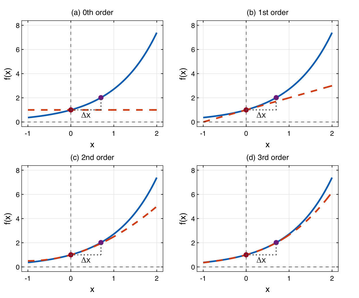
Taking \(\Delta x = 0.2\) in Eq. 1, the third-order Taylor polynomial is
\[ e^{x + 0.2} \approx e^{x} + e^{x}(0.2) + \frac{e^{x}}{2!}(0.2)^{2} + \frac{e^{x}}{3!}(0.2)^{3} \equiv P_3(\Delta x). \]
This approximation uses only the function and its derivatives at \(x\) up to third order, and it becomes increasingly accurate as \(\Delta x \to 0\). The progression from a zeroth-order (constant) approximation to a third-order (cubic) approximation is shown in Figure 1.
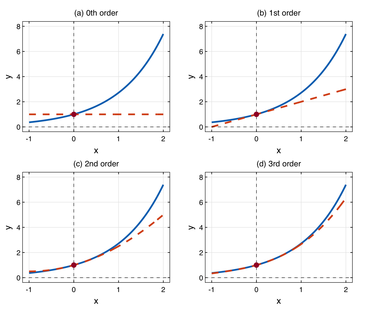
Alternatively, expanding \(e^{x}\) about \(a = 0\) (the Maclaurin series) and truncating at third order gives
\[ e^x \approx 1 + \frac{x}{1!} + \frac{x^{2}}{2!} + \frac{x^{3}}{3!} \equiv P_{3}(x), \]
which produces a finite-order approximation of \(e^{x}\) near the expansion point. As \(n\) grows, \(P_{n}(x)\) approximates \(e^{x}\) increasingly well:
- 0th order (constant): \(P_{0}(x) = 1\)
- 1st order (tangent line): \(P_{1}(x) = 1 + x\)
- 2nd order (adds curvature): \(P_{2}(x) = 1 + x + x^{2}/2!\)
- 3rd order and higher: progressively improve local accuracy.
The progression is illustrated in Figure 2.
2.2 Geometric interpretation of the second-order Taylor term
The second-order term \(\tfrac{1}{2} f''(a)(x-a)^{2}\) is often dismissed as an algebraic afterthought, but it has a crisp geometric reading that makes Itô’s lemma much easier to remember. The trick is to Taylor-expand not \(f\) itself but the area under \(f\): doing so turns every term of the expansion into a shape you can point at.
Fix a left endpoint \(x_{0}\) and define the running area
\[ F(x) \;\equiv\; \int_{x_{0}}^{x} f(t)\, dt, \tag{3}\]
so that \(F(x)\) measures the signed area under \(f\) from \(x_{0}\) out to the moving right endpoint \(x\). By the fundamental theorem of calculus,
\[ F'(x) = f(x), \qquad F''(x) = f'(x), \]
that is, the first derivative of the area is the height of the curve and the second derivative is the slope of the curve. Substituting into the second-order Taylor expansion of \(F\) about the base point \(a\) gives
\[ F(x) \;\approx\; F(a) \;+\; f(a)\,(x-a) \;+\; \tfrac{1}{2}\, f'(a)\,(x-a)^{2}. \tag{4}\]
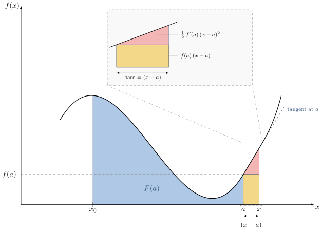
Each term on the right-hand side is a shape visible in Figure 3:
Zeroth order: \(F(a)\) (blue region). The area already accumulated up to the base point \(a\). It is the value of the area function at \(a\), before the endpoint moves.
First order: \(f(a)\,(x-a)\) (gold rectangle). If we naively pretend that \(f\) is constant and equal to \(f(a)\) on \([a, x]\), the extra area swept out as the endpoint moves from \(a\) to \(x\) is exactly a rectangle of height \(f(a)\) and base \((x-a)\). This is the linear estimate of the increment \(F(x) - F(a)\) — what a first-order Taylor expansion of \(F\) contributes.
Second order: \(\tfrac{1}{2}\, f'(a)\,(x-a)^{2}\) (pink triangle). The rectangle is systematically wrong whenever \(f\) is not flat: it underestimates the increment when \(f\) is rising (\(f'(a) > 0\)) and overestimates it when \(f\) is falling. Locally the curve is best replaced by its tangent line at \(a\), which lifts above the top of the rectangle by \(f'(a)(x-a)\) at the right endpoint. The triangle wedged between the top of the rectangle and the tangent line has base \((x-a)\) and height \(f'(a)(x-a)\), so its area is
\[ \tfrac{1}{2}\,\underbrace{(x-a)}_{\text{base}}\, \underbrace{f'(a)\,(x-a)}_{\text{height}} \;=\; \tfrac{1}{2}\, f'(a)\,(x-a)^{2}, \]
exactly the second-order term in Eq. 4.
In both panels of the figure the pink triangle is bounded above by the tangent line, and across \([a, x]\) the drawn curve lies along that tangent — which is exactly the substitution a second-order expansion makes. What it leaves out shows up just past \(x\), where the drawn curve bends away above the tangent and the two visibly separate. That widening gap holds everything left over — the cubic, quartic, and higher-order Taylor terms. At the step drawn in the figure the three pieces are correctly ordered: the triangle is 43% of the rectangle, and the sliver is 6% of the whole increment. As the step \((x-a)\) shrinks that ordering only sharpens, because the sliver vanishes faster than the pink triangle, which in turn vanishes faster than the gold rectangle. The triangle is therefore the dominant correction to the rectangle once linear information has been exhausted.
Two takeaways deserve emphasis. First, the second-order term is not a rounding error but the leading-order mismatch between the tangent line and a curve of nonzero curvature, and its size grows quadratically with the step \((x-a)\). Second, this same accounting argument — a linear “tangent” prediction plus a quadratic correction whose sign is set by the local curvature — reappears verbatim when we Taylor-expand the derivative price \(V(S_t, t)\) in Section 4. There the tangent piece is the option’s delta, \(\partial V/\partial S\), and the quadratic correction is exactly the \(\tfrac{1}{2}\, \sigma^{2} S_{t}^{2}\, \partial^{2} V/\partial S^{2}\) gamma term that survives Itô’s rules. The geometric picture is the same; only the object being expanded changes.
3 Itô’s Process
Consider a smooth function \(V\) depending on the state \(S_{t}\) and on time \(t\). Applying a second-order Taylor expansion as in Eq. 1 to \(V(S_t + \Delta S_t,\; t + \Delta t)\) about \((S_{t},t)\) yields
\[ \begin{aligned} V(S_t + \Delta S_t,\; t + \Delta t) \approx V(S_t, t) &+ \frac{\partial V}{\partial S}\,\Delta S_t + \frac{\partial V}{\partial t}\,\Delta t + \frac{1}{2}\frac{\partial^{2}V}{\partial S^{2}}\,(\Delta S_t)^{2} \\ &+ \frac{\partial^{2}V}{\partial S\,\partial t}\,\Delta S_t\,\Delta t + \frac{1}{2}\frac{\partial^{2}V}{\partial t^{2}}\,(\Delta t)^{2}, \end{aligned} \]
where all partial derivatives are evaluated at \((S_t, t)\) and higher-order terms are of smaller order (they will vanish once we apply Itô’s rules below). Define the increment
\[ \Delta V_t := V(S_t + \Delta S_t,\; t + \Delta t) - V(S_t, t). \]
Then
\[ \Delta V_t \approx \frac{\partial V}{\partial S}\,\Delta S_t + \frac{\partial V}{\partial t}\,\Delta t + \frac{1}{2}\frac{\partial^{2}V}{\partial S^{2}}\;(\Delta S_t)^{2} + \frac{\partial^{2}V}{\partial S\,\partial t}\;\Delta S_t\,\Delta t + \frac{1}{2}\frac{\partial^{2}V}{\partial t^{2}}\;(\Delta t)^{2}. \]
Formally replacing the finite increments by differentials,
\[ dV_t \approx \frac{\partial V}{\partial S}\,dS_t + \frac{\partial V}{\partial t}\, dt + \frac{1}{2}\frac{\partial^{2}V}{\partial S^{2}}\,(dS_t)^{2} + \frac{\partial^{2}V}{\partial S\,\partial t}\,dS_t\, dt + \frac{1}{2}\frac{\partial^{2}V}{\partial t^{2}}\,(dt)^{2}. \tag{5}\]
Up to this point the derivation is an ordinary Taylor expansion. Stochastic calculus enters when we specify the dynamics of \(S_t\) and apply Itô’s rules to the differentials \(dS_t\), \(dW_t\), and \(dt\).
3.1 Geometric Brownian motion
Assume that the underlying \(S_t\) (e.g., a stock price) follows the diffusion
\[ dS_{t} = \mu S_{t}\,dt + \sigma S_{t}\,dW_{t}, \tag{6}\]
where \(\mu\) is the drift (the instantaneous expected rate of return) and \(\sigma\) is the volatility, so that \(\sigma S_t\) is the instantaneous volatility of the stock price over the short interval \(dt\). The key stochastic ingredient is \(dW_t\), where \((W_t)_{t \ge 0}\) is a standard Wiener process.
3.2 The Wiener process
The Wiener process \((W_t)_{t \ge 0}\) (also called standard Brownian motion) is a continuous-time Markov stochastic process with zero drift and unit variance rate. Formally, it is characterised by two defining properties.
Normal increments. Over a small time interval \(dt\), the increment satisfies
\[ dW_t = \epsilon \sqrt{dt},\qquad \epsilon \sim \mathcal{N}(0,1). \]
Independent increments. The increments \(dW_t\) over non-overlapping intervals \(dt\) are mutually independent.
The first property implies that \(dW_t\) is normally distributed with
- \(\mathbb{E}[dW_t] = \sqrt{dt}\, \mathbb{E}[\epsilon] = 0\),
- \(\operatorname{Var}(dW_t) = dt\, \operatorname{Var}(\epsilon) = dt\),
- \(\sqrt{\operatorname{Var}(dW_t)} = \sqrt{dt}\).
The second property implies the Markov property: only the current value of the process is relevant for forecasting future increments.
4 Itô’s Lemma
Substituting Eq. 6 into Eq. 5 and applying the Itô rules
\[ (dt)^{2} = 0, \qquad (dW_{t})^{2} = dt, \qquad dt\,dW_{t} = 0, \]
we obtain
\[ \begin{aligned} dV_t &= \frac{\partial V}{\partial S}\,dS_t + \frac{\partial V}{\partial t}\,dt + \frac{1}{2}\frac{\partial^{2}V}{\partial S^{2}}\,(dS_t)^2 \\ &= \frac{\partial V}{\partial S}\,(\mu S_{t}\,dt + \sigma S_{t}\,dW_{t}) + \frac{\partial V}{\partial t}\,dt + \frac{1}{2}\frac{\partial^{2}V}{\partial S^{2}}\,(\mu S_{t}\,dt + \sigma S_{t}\,dW_{t})^2 \\ &= \frac{\partial V}{\partial S}\,(\mu S_{t}\,dt + \sigma S_{t}\,dW_{t}) + \frac{\partial V}{\partial t}\,dt + \frac{1}{2}\frac{\partial^{2}V}{\partial S^{2}}\,\bigl(\mu^2 S^2_{t}(dt)^2 + 2\mu \sigma S^2_{t}\,dt\,dW_{t} + \sigma^2 S^2_{t}\,(dW_{t})^2\bigr) \\ &= \frac{\partial V}{\partial S}\,(\mu S_{t}\,dt + \sigma S_{t}\,dW_{t}) + \frac{\partial V}{\partial t}\,dt + \frac{1}{2}\sigma^{2}S_{t}^{2}\frac{\partial^{2}V}{\partial S^{2}}\,dt \\ &= \Bigl(\frac{\partial V}{\partial S}\,\mu S_{t} + \frac{\partial V}{\partial t} + \frac{1}{2}\frac{\partial^{2}V}{\partial S^{2}}\sigma^{2}S_{t}^{2}\Bigr)dt + \frac{\partial V}{\partial S}\,\sigma S_{t}\,dW_{t}. \end{aligned} \tag{7}\]
This is the standard form of Itô’s lemma for a function of a single stochastic variable \(S_t\). Comparing Eq. 7 with the naive chain-rule expansion, the additional \(\tfrac{1}{2}\sigma^{2}S_{t}^{2}\, \partial^{2}V/\partial S^{2}\, dt\) term is exactly the Itô correction. Geometrically, it plays the same role as the pink triangle in Section 2.2: a quadratic correction whose sign is set by the local curvature of \(V\) in \(S\).
5 Black-Scholes(-Merton)
5.1 The delta-hedged portfolio and the PDE
The discrete-time version of Eq. 7 is
\[ \Delta V_t = \Bigl(\frac{\partial V}{\partial S}\,\mu S_{t} + \frac{\partial V}{\partial t} + \frac{1}{2}\frac{\partial^{2}V}{\partial S^{2}}\sigma^{2}S_{t}^{2}\Bigr)\Delta t + \frac{\partial V}{\partial S}\,\sigma S_{t}\,\Delta W_{t}, \tag{8}\]
where \(\Delta W_t = \epsilon \sqrt{\Delta t}\) with \(\epsilon \sim \mathcal{N}(0,1)\). It follows that a portfolio short one derivative and long \(\partial V/\partial S\) shares of the underlying can be constructed so that the Wiener term cancels. Concretely, define
\[ \begin{aligned} -1 &:\ \text{derivative} \\ +\,\frac{\partial V}{\partial S} &:\ \text{shares of the stock,} \end{aligned} \]
so that the value of the portfolio at time \(t\) is
\[ \Pi_t = -V(S_t,t) + \frac{\partial V(S_t,t)}{\partial S}\, S_t. \]
Over the short interval \(\Delta t\) its change is
\[ \Delta \Pi_t = -\,\Delta V_t + \frac{\partial V}{\partial S}\,\Delta S_t, \]
where
\[ \Delta S_t = \mu S_t \,\Delta t + \sigma S_t\, \Delta W_t. \]
Substituting Eq. 8 for \(\Delta V_t\) and the expression for \(\Delta S_t\),
\[ \begin{aligned} \Delta \Pi_t &= -\Bigl(\frac{\partial V}{\partial S}\,\mu S_{t} + \frac{\partial V}{\partial t} + \frac{1}{2}\frac{\partial^{2}V}{\partial S^{2}}\sigma^{2}S_{t}^{2}\Bigr)\Delta t - \frac{\partial V}{\partial S}\,\sigma S_{t}\,\Delta W_{t} \\ &\qquad + \frac{\partial V}{\partial S}\bigl(\mu S_t \,\Delta t + \sigma S_t\, \Delta W_t\bigr) \\ &= -\Bigl(\frac{\partial V}{\partial t} + \frac{1}{2}\frac{\partial^{2}V}{\partial S^{2}}\sigma^{2}S_{t}^{2}\Bigr)\Delta t. \end{aligned} \]
The \(\Delta W_t\) terms cancel, so over the interval \(\Delta t\) the portfolio is locally riskless: its change does not depend on \(\Delta W_t\). By no arbitrage it must earn the risk-free rate \(r\):
\[ \Delta \Pi_t = r\, \Pi_t\, \Delta t = r\Bigl(-V + \frac{\partial V}{\partial S}\, S_t\Bigr)\Delta t. \]
Equating the two expressions for \(\Delta \Pi_t\) and dividing by \(\Delta t\) yields
\[ -\Bigl(\frac{\partial V}{\partial t} + \frac{1}{2}\frac{\partial^{2}V }{\partial S^{2}}\sigma^{2}S_{t}^{2}\Bigr) = r\Bigl(-V + \frac{\partial V}{\partial S}\, S_t\Bigr), \]
which rearranges to the Black-Scholes PDE:
\[ \frac{\partial V}{\partial t} + \frac{1}{2}\sigma^{2}S^{2}\frac{\partial^{2}V}{\partial S^{2}} + r S \frac{\partial V}{\partial S} - rV = 0. \tag{9}\]
Eq. 9 has many solutions, one for each choice of boundary conditions. For a European call struck at \(K\) and maturing at \(T\), the terminal condition is
\[ V(S_T, T) = \max(S_T - K, 0), \]
and the PDE together with this boundary condition admits the closed-form solution
\[ C(S_t, t) = S_t\, N(d_1) - K e^{-r{(T-t)}}\, N(d_2), \tag{10}\]
with
\[ d_1 = \frac{\ln(S_t / K) + (r + \tfrac{1}{2}\sigma^2)(T-t)}{\sigma \sqrt{T-t}}, \qquad d_2 = d_1 - \sigma\sqrt{T - t}, \]
where \(N(\cdot)\) is the standard normal CDF.
5.2 Where do \(N(d_1)\) and \(N(d_2)\) come from?
The hedging argument shows that the value \(V(S,t)\) of any derivative written on \(S_t\) must satisfy the Black-Scholes PDE Eq. 9 together with the terminal condition imposed by the payoff. A key result from stochastic analysis, the Feynman-Kac theorem (Shreve 2004), states that the solution can be expressed as a discounted expectation under the risk-neutral measure \(\mathbb{Q}\) (Harrison and Pliska 1981). For a European call,
\[ V(S_t, t) = e^{-r(T-t)}\, \mathbb{E}^{\mathbb{Q}}\bigl[(S_T - K)^+ \mid S_t\bigr], \]
where under \(\mathbb{Q}\) the stock evolves according to
\[ dS_t = r S_t\, dt + \sigma S_t\, dW_t^{\mathbb{Q}}. \]
Solving this SDE (see Section 5.3) shows that \(S_T\) is lognormally distributed:
\[ S_T = S_t\exp\!\Bigl((r-\tfrac12\sigma^2)(T-t) + \sigma\sqrt{T-t}\,Z\Bigr),\qquad Z\sim N(0,1). \]
Writing the payoff as \((S_T - K)^+ = (S_T - K)\mathbf{1}_{\{S_T > K\}}\), the event \(\{S_T > K\}\) becomes a linear inequality in the standard normal variable \(Z\), and the expectation reduces to two Gaussian integrals:
\[ \begin{aligned} V(S_t, t) &= e^{-r(T-t)}\, \mathbb{E}^{\mathbb{Q}}\bigl[(S_T - K)^+ \mid S_t\bigr] \\ &= e^{-r(T-t)}\, \bigl(\underbrace{\mathbb{E}^{\mathbb{Q}}\bigl[S_T\, \mathbf{1}_{\{S_T > K\}} \mid S_t\bigr]}_{A} - K \underbrace{\mathbb{Q}\bigl(S_T > K \mid S_t\bigr)}_{B}\bigr). \end{aligned} \]
Solving for \(B\). Using the explicit form of \(S_T\),
\[ \begin{aligned} \mathbb{Q}(S_T > K \mid S_t) &= \mathbb{Q}\Bigl(S_t\exp\!\bigl((r-\tfrac{1}{2}\sigma^2)(T-t) + \sigma\sqrt{T-t}\,Z\bigr) > K\Bigr) \\ & = \mathbb{Q}\Bigl(Z > \frac{\ln(K / S_t) - (r-\tfrac{1}{2}\sigma^2)(T-t)}{\sigma\sqrt{T-t}}\Bigr) \\ & = \mathbb{Q}\Bigl(Z > -\frac{\ln(S_t / K) + (r-\tfrac{1}{2}\sigma^2)(T-t)}{\sigma\sqrt{T-t}}\Bigr) \\ & = \mathbb{Q}(Z > -d_2). \end{aligned} \]
Since \(Z \sim N(0,1)\) is symmetric about zero,
\[ B = \mathbb{Q}(S_T > K \mid S_t) = \mathbb{Q}(Z > -d_2) = \mathbb{Q}(Z < d_2) = N(d_2). \]
Solving for \(A\).
\[ \begin{aligned} \mathbb{E}^{\mathbb{Q}}\!\bigl[S_T\, \mathbf{1}_{\{S_T > K\}} \mid S_t\bigr] &= \mathbb{E}^{\mathbb{Q}}\!\Bigl[S_t \exp\!\bigl((r - \tfrac{1}{2}\sigma^2)(T - t) + \sigma\sqrt{T - t}\, Z\bigr)\, \mathbf{1}_{\{S_T > K\}} \mid S_t\Bigr] \\ &= S_t e^{(r - \tfrac{1}{2}\sigma^2)(T - t)}\, \mathbb{E}^{\mathbb{Q}}\!\bigl[e^{\sigma\sqrt{T - t}\, Z}\, \mathbf{1}_{\{Z > -d_2\}}\bigr]. \end{aligned} \]
The Gaussian integral
\[ \mathbb{E}\bigl[e^{aZ}\, \mathbf{1}_{\{Z > -d_2\}}\bigr] = \int_{-d_2}^{\infty} e^{az}\, \phi(z)\, dz, \qquad a = \sigma\sqrt{T - t}, \]
is evaluated by completing the square in the exponent. This yields
\[ \mathbb{E}\bigl[e^{aZ}\, \mathbf{1}_{\{Z > -d_2\}}\bigr] = e^{\tfrac{1}{2}a^2}\, N(d_1), \]
so that
\[ A = S_t\, e^{r (T - t)}\, N(d_1). \]
Substituting \(A\) and \(B\) back into the valuation formula reproduces the Black-Scholes call price:
\[ C(S_t, t) = S_t\, N(d_1) - K\, e^{-r(T-t)}\, N(d_2), \]
which matches Eq. 10. The put price follows by the same logic (or by put-call parity):
\[ P(S_t, t) = K\, e^{-r(T-t)}\, N(-d_2) - S_t\, N(-d_1). \]
5.3 Why is \(S_T\) lognormally distributed?
To solve the SDE under \(\mathbb{Q}\),
\[ dS_t = r S_t\, dt + \sigma S_t\, dW_t, \]
consider the process \(X_t = \ln S_t\). Applying Itô’s lemma to \(f(s) = \ln s\), for which
\[ f'(S_t) = \frac{1}{S_t}, \qquad f''(S_t) = -\frac{1}{S_t^2}, \]
we obtain
\[ dX_t = f'(S_t)\, dS_t + \tfrac{1}{2} f''(S_t)\, (dS_t)^2. \]
Substituting \(dS_t = r S_t\, dt + \sigma S_t\, dW_t\) and using the Itô rules \((dW_t)^2 = dt\), \((dt)^2 = 0\), \(dt\, dW_t = 0\),
\[ \begin{aligned} dX_t &= \frac{1}{S_t}(r S_t\, dt + \sigma S_t\, dW_t) + \frac{1}{2}\!\left(-\frac{1}{S_t^2}\right) \sigma^2 S_t^2\, dt \\ &= r\, dt + \sigma\, dW_t - \tfrac{1}{2}\sigma^2\, dt \\ &= \bigl(r - \tfrac{1}{2}\sigma^2\bigr)\, dt + \sigma\, dW_t. \end{aligned} \]
Integrating from \(t\) to \(T\),
\[ \int_t^T dX_s = \int_t^T \bigl(r - \tfrac{1}{2}\sigma^2\bigr)\, ds + \int_t^T \sigma\, dW_s, \]
the left-hand side equals \(X_T - X_t = \ln S_T - \ln S_t\), so
\[ \ln S_T = \ln S_t + \bigl(r - \tfrac{1}{2}\sigma^2\bigr)(T-t) + \sigma\,(W_T - W_t). \]
Exponentiating,
\[ S_T = S_t \exp\!\Bigl( (r - \tfrac{1}{2}\sigma^2)(T-t) + \sigma (W_T - W_t) \Bigr). \]
Finally, using the Brownian-increment property \(W_T - W_t \sim N(0, T - t)\) (see the callout in Section 6), we may write \(W_T - W_t = \sqrt{T-t}\, Z\) with \(Z \sim N(0,1)\), so that
\[ S_T = S_t \exp\!\Bigl( (r - \tfrac{1}{2}\sigma^2)(T-t) + \sigma\sqrt{T-t}\,Z \Bigr),\qquad Z\sim N(0,1). \]
This shows that \(S_T\) is lognormally distributed — equivalently, that \(\ln S_T\) is normally distributed — with mean \(\ln S_t + (r - \tfrac{1}{2}\sigma^2)(T-t)\) and variance \(\sigma^{2}(T-t)\).
TipNormal representation of Brownian increments
The increment of a standard Brownian motion satisfies
\[ W_T - W_t \sim N(0, T - t) \]
for all \(0 \le t < T\). This is one of the defining properties of Brownian motion. If \(X \sim N(0, \sigma^2)\), then there exists a standard normal \(Z \sim N(0,1)\) such that
\[ X = \sigma Z, \]
because
\[ \operatorname{Var}(\sigma Z) = \sigma^2 \operatorname{Var}(Z) = \sigma^2. \]
Applying this fact to the Brownian increment with variance \(T-t\), we write
\[ W_T - W_t = \sqrt{T-t}\, Z, \qquad Z \sim N(0,1). \]
This is simply a reparameterisation of a normal random variable with variance \(T-t\) in terms of a standard normal variable.
6 Conclusion
Combining a second-order Taylor expansion with Itô’s rules yields Itô’s lemma, and applying it to the value of a derivative \(V(S_t, t)\) produces a diffusion whose \(dW_t\) component can be eliminated by a delta-hedged portfolio. The resulting local no-arbitrage condition is the Black-Scholes PDE Eq. 9, and evaluating the risk-neutral expectation implied by Feynman-Kac under the lognormal law of \(S_T\) delivers the closed-form call price Eq. 10. Extensions — dividends, stochastic volatility, early exercise, jumps — follow the same three-step recipe: pick a dynamics, apply Itô’s lemma, and enforce local no-arbitrage after constructing an appropriate hedged portfolio.
References
Black, Fischer, and Myron Scholes. 1973. “The Pricing of Options and Corporate Liabilities.” Journal of Political Economy 81 (3): 637–54.
Harrison, J. Michael, and Stanley R. Pliska. 1981. “Martingales and Stochastic Integrals in the Theory of Continuous Trading.” Stochastic Processes and Their Applications 11 (3): 215–60.
Hull, John C. 2021. Options, Futures, and Other Derivatives. 11th ed. Pearson.
Itô, Kiyosi. 1951. “On Stochastic Differential Equations.” Memoirs of the American Mathematical Society 4: 1–51.
Merton, Robert C. 1973. “Theory of Rational Option Pricing.” The Bell Journal of Economics and Management Science 4 (1): 141–83.
Shreve, Steven E. 2004. Stochastic Calculus for Finance II: Continuous-Time Models. Springer.