Financial Information Theory

These notes distill Financial Information Theory into a single algebraic fact: Jensen’s inequality, \(\mathbb{E}[\ln X] \le \ln \mathbb{E}[X]\). Each of the five substantive sections applies the same concavity in a different form. Section 2 turns it into the volatility-drag identity \(\mu - \sigma^{2}/2\) and defines Shannon entropy as expected surprisal. Section 3 promotes it to the log-optimality of Kelly–Latané portfolios and to the maximum-entropy principle for agnostic asset allocation. Section 4 recasts it as the non-negativity of Kullback–Leibler divergence, which is at once the rate at which a wrong belief burns compounded wealth and the per-symbol overhead of compressing \(P\) with a code matched to \(Q\). The same section generalizes correlation to mutual information and transfer entropy. Section 5 identifies the Kelly growth rate with Shannon channel capacity and reads Kelly betting as reliable communication over a noisy channel. Section 6 grounds cross-entropy loss, the information bottleneck, and the evidence lower bound used in generative market simulators. The notes are terse, self-contained, and assume measure-theoretic probability and elementary asset pricing.
information theory, entropy, Kelly criterion, mutual information, log-optimal portfolio
1 Introduction
Financial information theory is the systematic application of a single concave-function inequality to problems in asset pricing, portfolio choice, and market forecasting. Given a concave function \(\phi\) and a random variable \(X\) with finite mean, Jensen’s inequality asserts that:
\[ \mathbb{E}[\phi(X)] \le \phi(\mathbb{E}[X]), \tag{1}\]
with equality if and only if \(X\) is almost surely constant or \(\phi\) is affine on the support of \(X\) (Rockafellar 1970). Every result in these notes follows from Eq. 1 applied to \(\phi = \ln\) and a well-chosen random variable. The five sections that follow are that one identity in five forms.
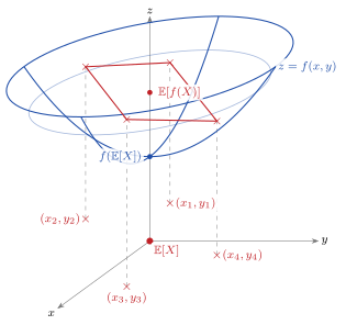
Figure 1 draws the inequality in its convex form, \(f(\mathbb{E}[X]) \le \mathbb{E}[f(X)]\), which is the version that makes the geometry easiest to see. Let \(f\) be convex on \(\mathbb{R}^{2}\) and let \(X\) take four values \((x_{i}, y_{i})\) with equal probability. Each realization lifts to a point on the surface \(z = f(x, y)\), and the chords joining those four points span a flat sheet strictly above the bowl. The average height \(\mathbb{E}[f(X)]\) is the centre of mass of that sheet, so it sits above the single surface point \(f(\mathbb{E}[X])\) directly beneath it. Reflecting the picture turns the bowl into a dome, reverses every inequality, and recovers Eq. 1.
Two features of the figure matter later. First, nothing depends on dimension: \(X\) lives in \(\mathbb{R}^{2}\) here only because a surface is easier to draw than a curve is to interpret, and the same chord-above-surface argument runs unchanged in \(\mathbb{R}^{n}\) or in a space of distributions. Second, the vertical gap between the two marked heights is what every section below names. It is called volatility drag, entropy deficit, relative entropy, or foregone growth depending on the form it takes, and it is always the same gap.
The first form is volatility drag. Because the logarithm is concave, the expected log return is bounded above by the log of the expected return, and the wedge between them is essentially variance (Section 2). The second is entropy. The expected surprisal \(\mathbb{E}[-\ln p(X)]\) attains its global maximum at the uniform distribution, which pins down the natural unit of uncertainty (Section 2) and becomes an allocation rule in Section 3. The third is divergence. The Kullback–Leibler distance \(D(P \parallel Q) = \mathbb{E}_{P}[\ln (p/q)]\) is non-negative and vanishes only at \(P = Q\). Its value equals both the per-period wealth-growth cost of betting on the wrong distribution and the per-symbol coding overhead of compressing \(P\) with a code matched to \(Q\) (Section 4). The fourth is capacity. The maximum log-growth of a portfolio equals the mutual information between the trader’s private signal and the market outcome, in exact analogy with Shannon’s channel-coding theorem (Section 5). The fifth is the ELBO. The log-likelihood of any latent-variable market model is bounded below by the evidence lower bound that generative networks optimize, again by Jensen (Section 6).
The notes are terse by design. Section 2 through Section 6 take the forms in turn. Each states its inequality as a proposition or theorem, sketches the proof, and closes with one financial reading. Identities used repeatedly (Gibbs, log-sum, data-processing, Fano) are collected in Appendix A.
2 The Root Split: Volatility Drag and Entropy
2.1 Volatility drag from Jensen
Wealth compounds multiplicatively, so terminal wealth depends on the average of each period’s log return rather than on the average of the return itself. The gap between the two averages is the first concrete form of the concavity that organizes these notes.
Fix a horizon of one period and let \(R > 0\) denote the gross return on a risky asset over that period. The arithmetic mean \(\mathbb{E}[R]\) tallies paper returns, what an investor earns by rebalancing back to the same dollar stake every period. The geometric mean \(\exp\{\mathbb{E}[\ln R]\}\) tallies compound growth, what a buy-and-hold dollar actually experiences. The two coincide only when \(R\) is deterministic.
The canonical thought experiment makes the wedge visible without any calculus. Let a dollar go up 50 percent and then down 50 percent, in either order and each with probability \(\tfrac{1}{2}\). The arithmetic average of the two gross returns \(\{1.5,\, 0.5\}\) is exactly one, suggesting break-even. Yet the two-period product is \(1.5 \times 0.5 = 0.75\), a 25 percent loss on the invested dollar. Volatility alone, with zero drift, destroyed a quarter of the capital. The asymmetry is baked into the logarithm: a 50 percent loss requires a 100 percent gain to recover, so symmetric arithmetic returns are systematically asymmetric in compound terms.
Jensen’s inequality applied to the concave function \(\phi = \ln\) formalises the phenomenon,
\[ \mathbb{E}[\ln R] \;\le\; \ln \mathbb{E}[R], \tag{2}\]
with equality only in the degenerate case. Compound growth always lags paper returns, and the gap widens with dispersion. The size of the gap admits a clean second-order expansion.
Let \(R = 1 + r\) with \(\mathbb{E}[r] = \mu\) and \(\operatorname{Var}(r) = \sigma^{2}\). For small \(\mu\) and \(\sigma\),
\[ \mathbb{E}[\ln R] \;=\; \mu - \tfrac{1}{2}\sigma^{2} + O\!\bigl(\mu^{2},\, \mathbb{E}[|r|^{3}]\bigr). \tag{3}\]
Proof. Sketch. Expand \(\ln(1+r) = r - r^{2}/2 + r^{3}/3 - \cdots\) and take expectations. The linear term contributes \(\mu\), the quadratic term contributes \(-\tfrac{1}{2}(\mu^{2} + \sigma^{2})\), and for small \(\mu\) the \(\mu^{2}\) piece is second-order relative to \(\sigma^{2}\).
The \(\sigma^{2}/2\) term is the volatility drag. It is a direct tax on compound growth equal to half the return variance, which gives variance a cost beyond the risk that diversification addresses. The same concavity reappears as Shannon entropy in the next subsection, as Kullback–Leibler divergence in Section 4, and as the Kelly ceiling in Section 5.
Eq. 3 has a direct financial reading. An expected return of 20 percent with volatility of 20 percent compounds at roughly \(0.20 - \tfrac{1}{2}(0.20)^{2} = 0.18\) per period, not 0.20. Double the volatility to 40 percent and the drag quadruples to eight percentage points, dragging compound growth down to 12 percent. Halve the volatility to 10 percent and the tax is just 50 basis points. The scaling is quadratic in \(\sigma\), which is why the marginal cost of the last unit of risk grows faster than the marginal reward of the last unit of expected return. That observation underlies the Kelly criterion. In continuous time the correction becomes exact: a geometric Brownian motion \(dS/S = \mu\, dt + \sigma\, dW\) has log-price drift \(\mu - \sigma^{2}/2\) by Itô’s lemma (Merton 1969; Luenberger 1998).
2.2 Shannon entropy as expected surprisal
The same concavity underwrites the mathematical definition of uncertainty. Let \(X\) be a discrete random variable representing a market state (up, down, flat, or any finer partition) drawn from a true distribution \(p\) on a finite alphabet \(\mathcal{X}\). The surprisal of an outcome \(X = x\) is:
\[ h(x) \;=\; \ln\!\bigg(\frac{1}{p(x)}\bigg) \;=\; -\ln p(x). \tag{4}\]
A certain event (\(p(x) = 1\)) carries zero surprisal, and an event of vanishing probability carries unbounded surprisal, so surprisal measures the improbability of what actually happened.
2.2.1 Defining entropy
The expected surprisal across all outcomes defines the Shannon entropy \(H(X)\), the average unpredictability of the system:
\[ H(X) \;=\; -\sum_{x \in \mathcal{X}} p(x) \ln p(x) \;=\; \mathbb{E}\bigl[-\ln p(X)\bigr]. \tag{5}\]
When is a market completely unpredictable? Intuition says: when every outcome is equally likely. Jensen’s inequality applied to \(\phi = \ln\) and the random variable \(1/p(X)\) proves it,
\[ H(X) \;=\; \mathbb{E}\!\Big[\ln \tfrac{1}{p(X)}\Big] \;\le\; \ln \mathbb{E}\!\Big[\tfrac{1}{p(X)}\Big], \tag{6}\]
and the expectation on the right collapses algebraically: \(\mathbb{E}[1/p(X)] = \sum_{x} p(x)\cdot 1/p(x) = |\mathcal{X}|\). Substituting back gives a hard ceiling on uncertainty,
\[ H(X) \;\le\; \ln |\mathcal{X}|, \tag{7}\]
with equality attained at the uniform distribution (Shannon 1948; Cover and Thomas 2006).
Eq. 7 does two things. It fixes the natural unit of uncertainty, the “nat”, which is the surprise carried by an event of probability \(1/e \approx 36.8\%\), and every later quantity is measured in it: mutual information is a relative entropy, Kelly capacity a mutual information, and generative model loss a cross entropy. It also motivates the maximum entropy principle (Jaynes 1957), taken up in Section 3. Faced with an asset whose full law is unknown, the least presumptuous benchmark is the distribution that maximizes entropy subject only to the constraints one is willing to impose. Fixing the mean and variance, for instance, forces a Gaussian.
For financial time series the alphabet is rarely fixed. Continuous returns replace the sum in Eq. 5 by an integral and yield differential entropy \(h(X) = -\int f(x) \ln f(x)\, dx\), which loses non-negativity but keeps its convex-analytic role. Both discrete and differential entropies are strictly concave functionals of the underlying law, a fact used repeatedly below.
3 Quantifying States and Assets
3.1 Log-optimal portfolios
Consider \(n\) risky assets with random gross returns \(\mathbf{R} = (R_{1}, \ldots, R_{n})\) and a portfolio weight vector \(\mathbf{b}\) on the simplex \(\{\mathbf{b} \ge 0,\; \sum_{i} b_{i} = 1\}\). The portfolio return over one period is \(\mathbf{b}^{\prime}\mathbf{R}\). Over \(T\) i.i.d. periods, the compound wealth \(S_{T}(\mathbf{b}) = \prod_{t=1}^{T} \mathbf{b}^{\prime}\mathbf{R}_{t}\) satisfies, by the strong law of large numbers,
\[ \tfrac{1}{T}\, \ln S_{T}(\mathbf{b}) \;\xrightarrow{\text{a.s.}}\; \mathbb{E}\bigl[\ln \mathbf{b}^{\prime}\mathbf{R}\bigr]. \tag{8}\]
The maximizer of the right-hand side over \(\mathbf{b}\) defines the log-optimal portfolio, \(\mathbf{b}^{\star}\).
The log-optimal portfolio dominates every alternative in the sense that
\[ \limsup_{T \to \infty} \frac{1}{T} \ln \frac{S_{T}(\mathbf{b})}{S_{T}(\mathbf{b}^{\star})} \;\le\; 0 \quad \text{almost surely,} \tag{9}\]
for every portfolio \(\mathbf{b}\) on the simplex, with equality if and only if \(\mathbf{b} = \mathbf{b}^{\star}\) almost surely (Kelly 1956; Breiman 1961; Algoet and Cover 1988).
Proof. Sketch. Kuhn–Tucker conditions at \(\mathbf{b}^{\star}\) give \(\mathbb{E}[R_{i}/\mathbf{b}^{\star\prime}\mathbf{R}] \le 1\) with equality on the support of \(\mathbf{b}^{\star}\). Any alternative \(\mathbf{b} \ge 0\) with \(\sum_{i} b_{i} = 1\) then satisfies \(\mathbb{E}[\mathbf{b}^{\prime}\mathbf{R}/\mathbf{b}^{\star\prime}\mathbf{R}] \le 1\). Jensen applied to the log gives \(\mathbb{E}[\ln(\mathbf{b}^{\prime}\mathbf{R}/\mathbf{b}^{\star\prime}\mathbf{R})] \le 0\), and Eq. 8 converts the expectation into the almost sure statement of Eq. 9.
Eq. 9 is stronger than the statement that the log-optimal rule maximizes expected log wealth. It says that log-optimal wealth almost surely outgrows any competitor’s over long horizons. Latané (1959) obtained the same result independently and called it the geometric-mean criterion. Log-optimal weights need not be non-negative when short-selling is allowed (Algoet and Cover 1988), but the domination result carries over unchanged.
3.2 Maximum-entropy allocation
Log-optimality presumes a known return distribution. When the distribution is not known, the principle of maximum entropy (Jaynes 1957) offers a canonical default. Given moment constraints \(\mathbb{E}_{p}[T_{k}(X)] = \tau_{k}\) for \(k = 1, \ldots, K\), the entropy-maximizing distribution takes exponential-family form
\[ p^{\star}(x) \;=\; \frac{1}{Z(\boldsymbol{\lambda})} \exp\!\Big\{\sum_{k=1}^{K} \lambda_{k}\, T_{k}(x)\Big\}, \tag{10}\]
where the Lagrange multipliers \(\lambda_{k}\) are pinned down by the constraints. Two special cases carry all the intuition. Fixing only the support recovers the uniform distribution, so MaxEnt with zero moment constraints reduces to Eq. 7. Fixing the mean and variance on \(\mathbb{R}\) recovers the Gaussian.
In portfolio choice the constraints are typically the first two moments of asset returns. MaxEnt allocation then produces the same mean-variance tangent portfolio one obtains from a Gaussian prior, with a derivation that commits only to the constraints the analyst is willing to impose (Meucci 2005).
3.3 Market randomness metrics
The entropy \(H\) measures uncertainty in a single-period distribution. The empirical randomness of a realized time series, meaning the rate at which past realizations forecast future ones, is measured by approximate entropy \(\operatorname{ApEn}(m, r)\) (Pincus 1991) and permutation entropy \(\operatorname{PE}\) (Bandt and Pompe 2002). Both count the frequency of length-\(m\) patterns in a realized sequence and take a normalized log. Both diagnose a market state as close to i.i.d. when their value approaches \(\ln (\text{alphabet size})\) and as highly predictable when they collapse toward zero.
For high-frequency order-book data, permutation entropy is model-free (no binning of returns is required) and computationally cheap, which makes it a common regime-detection input in the microstructure literature (Zunino et al. 2010). Both metrics are diagnostic here: they answer how random a state is. The next section uses divergence and mutual information to answer how connected two states are.
4 Non-Linear Channels
4.1 Kullback–Leibler divergence as wealth destruction
Given two probability laws \(P\) and \(Q\) on the same space with \(P \ll Q\), the relative entropy (or Kullback–Leibler divergence) is
\[ D(P \parallel Q) \;=\; \mathbb{E}_{P}\!\Big[\ln \tfrac{dP}{dQ}\Big] \;=\; \int p(x) \ln \tfrac{p(x)}{q(x)}\, dx. \tag{11}\]
Jensen’s inequality applied to \(\phi = -\ln\) and \(Y = dQ/dP\) delivers Gibbs’ inequality
\[ D(P \parallel Q) \;=\; -\mathbb{E}_{P}\!\Big[\ln \tfrac{dQ}{dP}\Big] \;\ge\; -\ln \mathbb{E}_{P}\!\Big[\tfrac{dQ}{dP}\Big] \;=\; 0, \tag{12}\]
with equality if and only if \(P = Q\) almost everywhere (Kullback and Leibler 1951; Cover and Thomas 2006). Relative entropy is asymmetric and violates the triangle inequality, so it is not a metric. Positivity is what earns it the “distance” label.
The financial content of Eq. 12 is the cost of a wrong model. In the archetypal horse-race setting (finite outcome space with pari-mutuel odds equal to the reciprocal of the true probabilities), a gambler betting according to belief \(Q\) instead of the truth \(P\) suffers a per-period wealth-growth deficit of exactly
\[ W_{P}(P) - W_{P}(Q) \;=\; D(P \parallel Q). \tag{13}\]
Eq. 13 makes the “distance” heuristic for \(D\) operational: \(D(P \parallel Q)\) is the number of nats of wealth growth lost per period by acting on the wrong distribution (Thorp 1971; Cover and Thomas 2006, Ch. 6).
The identity has a twin reading in source coding. For any complete prefix code on the alphabet \(\mathcal{X}\) with lengths \(\ell(x)\) in nats, Kraft’s inequality lets us write \(\ell(x) = -\ln q(x)\) for some probability \(q\). The expected code length under source \(P\) then decomposes as
\[ \mathbb{E}_{P}[\ell(X)] \;=\; -\mathbb{E}_{P}[\ln q(X)] \;=\; H(P) + D(P \parallel Q), \tag{14}\]
so the excess length above the Shannon floor \(H(P)\) equals the same \(D(P \parallel Q)\) that appeared in Eq. 13. Nats of wealth burned by betting on belief \(Q\) and nats of encoding overhead paid for a \(Q\)-matched code are the same number, which makes Shannon’s 1948 source-coding theorem and Kelly’s 1956 investment identity one algebraic fact stated in two languages.
4.2 Mutual information vs. correlation
For two random variables \(X\) and \(Y\) with joint law \(P_{XY}\) and marginals \(P_{X}, P_{Y}\), the mutual information is
\[ I(X ; Y) \;=\; D(P_{XY} \parallel P_{X} \otimes P_{Y}) \;=\; H(X) - H(X \mid Y). \tag{15}\]
Gibbs makes \(I(X ; Y) \ge 0\), with equality if and only if \(X\) and \(Y\) are independent. Unlike Pearson correlation, mutual information captures any form of statistical dependence. A quadratic link \(Y = X^{2}\) with \(X\) zero-mean, for instance, has exactly zero linear correlation with \(X\) yet is recovered from it deterministically. Mutual information registers that dependence in full and correlation registers none (Granger and Lin 1994).
Mutual information subsumes correlation cleanly under the joint Gaussian assumption. If \((X, Y)\) is bivariate normal with linear correlation \(\rho\),
\[ I(X ; Y) \;=\; -\tfrac{1}{2} \ln(1 - \rho^{2}). \tag{16}\]
The two quantities are monotonically related in that case and interchangeable. Beyond the Gaussian world they diverge, and empirical estimates of \(I(X; Y)\) from copulas or \(k\)-nearest-neighbor plug-ins (Kraskov et al. 2004) regularly detect non-linear links in equity, foreign-exchange, and macro time series that correlation misses.
4.3 Transfer entropy
Mutual information is symmetric, \(I(X ; Y) = I(Y ; X)\), so it cannot say whether \(X\) drives \(Y\) or the reverse. Transfer entropy (Schreiber 2000) restores directionality by conditioning on the past of the target. For time series \(X_{t}\) and \(Y_{t}\) with pasts \(X_{t}^{(k)}, Y_{t}^{(\ell)}\),
\[ T_{X \to Y} \;=\; I\!\bigl(Y_{t+1} \,;\, X_{t}^{(k)} \,\bigm|\, Y_{t}^{(\ell)}\bigr), \tag{17}\]
which measures the reduction in uncertainty of \(Y_{t+1}\) provided by the past of \(X\), over and above what the past of \(Y\) already provides. Transfer entropy is non-negative (Gibbs again) and asymmetric in the two series.
The financial reading is Granger causality without the linear-VAR restriction. Transfer entropy from an order-book imbalance series to a mid-price series measures directional information flow at all lags and all functional forms, which is how informed trading and lead–lag relationships across exchanges are detected (Dimpfl and Peter 2013).
5 Channel Capacity and Position Sizing
5.1 Kelly betting as reliable communication
Kelly (1956) set out to compute the optimal bet size on a horse race given a noisy tip. Given true race probabilities \(P\) over outcomes \(X\), tips \(Y\) with joint law \(P(X, Y)\), and pari-mutuel odds equal to the reciprocal of the true probabilities, he showed that the maximum log-growth rate of wealth under any betting scheme is exactly the mutual information between tip and outcome:
\[ W^{\star} \;=\; I(X ; Y). \tag{18}\]
Shannon (1948) had proven a decade earlier that the maximum reliable communication rate over a noisy channel with input \(X\) and output \(Y\) is \(C = \max_{P_{X}} I(X ; Y)\), the channel capacity. Kelly’s growth rate and Shannon’s capacity coincide because the noisy channel and the noisy tip are the same object (Cover and Thomas 2006, Ch. 6).
For a two-outcome bet with true win probability \(p\), fair odds \(b : 1\), and no side information, Eq. 18 collapses to
\[ W^{\star}(f) \;=\; p \ln(1 + b f) + (1 - p) \ln(1 - f), \tag{19}\]
maximized at the Kelly fraction \(f^{\star} = (pb - q)/b\) with \(q = 1 - p\). Under fair odds (\(b = q/p\)) the maximum equals \(\ln 2 - H(X)\), which is the capacity \(\ln 2 - H(p)\) of a binary symmetric channel, exactly as Eq. 18 requires.
5.2 Capacity as a hard ceiling
Eq. 18 is a ceiling rather than a target. Betting more than the Kelly fraction means leveraging beyond the capacity of the private information, and the concavity that set the ceiling then works against the bettor. Growth rate as a function of leverage \(\ell\) (with \(f = \ell f^{\star}\)) is concave with a maximum at \(\ell = 1\), so a second-order expansion around the optimum gives
\[ W(\ell f^{\star}) \;\approx\; W^{\star} + \tfrac{1}{2}\, W^{\prime\prime}(f^{\star})\, {f^{\star}}^{2}\, (\ell - 1)^{2}, \tag{20}\]
with \(W^{\prime\prime}(f^{\star}) < 0\) pinning the decay symmetrically on either side. The growth rate crosses zero around \(\ell = 2\) (double Kelly) and diverges to \(-\infty\) beyond, once the almost-sure lower tail of \(\ln R\) dominates (MacLean et al. 2011). Practitioners routinely bet at fractional Kelly, \(\ell \in [0.25, 0.5]\), to insulate against estimation error in \(f^{\star}\) (Thorp 2006).
5.3 Information-theoretic portfolio networks
Correlation matrices give the standard input to hierarchical clustering and minimum-spanning-tree portfolio construction (Mantegna 1999). Replacing correlation with an information-theoretic distance rescues the construction from its Gaussian assumption. The variation of information (Meilă 2007)
\[ V(X, Y) \;=\; H(X, Y) - I(X ; Y) \;=\; H(X \mid Y) + H(Y \mid X) \tag{21}\]
is a proper metric on random variables and satisfies the triangle inequality. Substituting \(V\) for \(1 - |\rho|\) in a single-linkage clustering routine yields asset classes defined by shared non-linear structure rather than by shared exposure to a common linear factor.
6 Modern Generative Quant AI
6.1 Cross-entropy as a compression floor
The Kullback–Leibler decomposition rewrites divergence in terms of an entropy and a cross-entropy:
\[ D(P \parallel Q) \;=\; H(P, Q) - H(P), \qquad H(P, Q) \;:=\; -\mathbb{E}_{P}\bigl[\ln q(X)\bigr]. \tag{22}\]
Non-negativity of \(D\) implies \(H(P, Q) \ge H(P)\), so cross entropy is bounded below by the entropy of the true source. Operationally, \(H(P, Q)\) is the average number of nats needed to encode samples from \(P\) using a code matched to \(Q\), and \(H(P)\) is the Shannon floor that no code can undercut (Shannon 1948; Cover and Thomas 2006, Ch. 5). Minimizing cross entropy is therefore training a compressor with the model class as code book, and Eq. 22 gives the compression limit. A classifier trained on the negative log-likelihood of held-out labels under a model \(Q_{\theta}\) cannot drive the loss below \(H(P)\). When the loss stalls at a strictly positive value, either the model class does not contain the truth or the label distribution is genuinely stochastic, and the two cases are told apart only by enlarging the model class and seeing whether the loss falls further.
For financial forecasters the cross-entropy floor is a numerical estimate of the irreducible uncertainty in the outcome. A daily direction-of-return classifier on an efficient equity index cannot achieve loss below \(\ln 2 \approx 0.69\) nats, the entropy of a fair binary label. Reports of validation losses well below this floor almost always reflect label leakage.
6.2 The information bottleneck
Tishby and Zaslavsky (2015) formalize representation learning as a rate–distortion problem. Given input \(X\) and label \(Y\), a stochastic encoder \(T = f(X)\) solves
\[ \min_{T} \; I(X ; T) - \beta\, I(T ; Y), \tag{23}\]
where \(\beta > 0\) trades off compression against relevance. The optimal representation \(T^{\star}\) is a sufficient statistic for \(Y\) in the limit \(\beta \to \infty\) and a minimally sufficient one at finite \(\beta\). The data-processing inequality (Appendix A, Row 4) forces \(I(T ; Y) \le I(X ; Y)\) for any encoder \(T = f(X)\), so compression can only destroy information about \(Y\), never create it. The information bottleneck picks the encoder that destroys the least under a given compression budget, tracing out the Pareto frontier of the plane \((I(X ; T),\, I(T ; Y))\) that the data-processing bound pins from above. Applied to alternative financial data such as news, social media, and macro dashboards, it extracts the low-dimensional signal \(T\) that preserves predictive power for \(Y\) (say, next-week returns) while discarding source-specific noise.
6.3 The evidence lower bound
Generative market simulators (variational autoencoders and diffusion models trained on historical returns) face an intractable marginal likelihood \(\log p_{\theta}(x) = \log \int p_{\theta}(x, z)\, dz\). Jensen supplies the standard lower bound. For any variational law \(q_{\phi}(z \mid x)\),
\[ \log p_{\theta}(x) \;=\; \log \mathbb{E}_{q_{\phi}}\!\Big[\tfrac{p_{\theta}(x, z)}{q_{\phi}(z \mid x)}\Big] \;\ge\; \mathbb{E}_{q_{\phi}}\!\bigl[\ln p_{\theta}(x, z) - \ln q_{\phi}(z \mid x)\bigr] \;=:\; \mathcal{L}(x;\theta,\phi), \tag{24}\]
the evidence lower bound (Jordan et al. 1999; Kingma and Welling 2014). Joint maximization of \(\mathcal{L}\) over \((\theta, \phi)\) simultaneously fits the generative model and refines the approximating posterior. Diffusion models specialize Eq. 24 to a fixed forward-noise process, replacing \(q_{\phi}\) with a Gaussian kernel and reducing ELBO maximization to a sequence of denoising regressions (Ho et al. 2020).
7 Conclusion
Five sections, one inequality. Volatility drag is Jensen on the log return, entropy is Jensen on the log density, Kullback–Leibler divergence is Jensen on the log-likelihood ratio, Kelly capacity is Jensen on log wealth, and the ELBO is Jensen on the marginal likelihood of a latent-variable model. In each case the concavity of the logarithm turns an inequality into a design principle: bet the log-optimal fraction, allocate at maximum entropy, cluster by variation of information, train against a cross-entropy floor. That shared structure is what lets one compact algebraic fact carry so much financial content.
Two extensions are worth flagging. The first is risk-neutral: the log-optimal portfolio corresponds to a specific choice of numéraire, and its counterpart under the equivalent martingale measure recovers the standard no-arbitrage machinery (Platen and Heath 2006). The second is robust: replacing Jensen with a \(\phi\)-divergence generalization gives distributionally robust portfolio choice and connects the Kelly criterion to modern robust control (Ben-Tal et al. 2009). Both rest on the same single inequality.
References
Appendix A Key Inequalities
Every result in Section 2 through Section 6 reduces to one of the five inequalities gathered in Table 1, each stated in its most general form. Specializations to the log or to specific measures are given inline where they are used in the main text.
| Name | Statement | First used in |
|---|---|---|
| Jensen | \(\mathbb{E}[\phi(X)] \le \phi(\mathbb{E}[X])\), \(\phi\) concave | Eq. 1 |
| Gibbs | \(D(P \parallel Q) \ge 0\), equality iff \(P = Q\) | Eq. 12 |
| Log-sum | \(\sum_{i} a_{i} \ln (a_{i}/b_{i}) \ge \bigl(\sum_{i} a_{i}\bigr) \ln \bigl(\sum_{i} a_{i} / \sum_{i} b_{i}\bigr)\) | proof of Eq. 12 |
| Data processing | \(X \to Y \to Z\) Markov \(\Rightarrow I(X ; Z) \le I(X ; Y)\) | Eq. 23 |
| Fano | \(H(P_{e}) + P_{e} \ln (|\mathcal{X}| - 1) \ge H(X \mid Y)\) | converse of Eq. 18 |
Jensen (Row 1) is the parent of the other four. Gibbs (Row 2) is Jensen applied to a log-likelihood ratio. The log-sum inequality (Row 3) is the discrete form of Gibbs and the workhorse for chain-rule and convexity proofs of the mutual information decomposition. The data-processing inequality (Row 4) states that no post-processing of \(Y\) can recover information about \(X\) that \(Y\) already lost, which is what pins down sufficiency for the information bottleneck. Fano’s inequality (Row 5) lower-bounds the error probability of any decoder in terms of the conditional entropy of the source and provides the converse to Eq. 18 that turns Kelly capacity into a hard information-theoretic ceiling.